ml.clustering.kmedoids

2.0.2

This package provides a Quantum K-Medoids clustering algorithm.

It provides a Python implementation of a QUBO based K-Medoids clustering algorithm.

The implementation (see the QKMedoids class) has been done in accordance with the scikit-learn estimator API, which means that the clustering algorithm can be used as any other scikit-learn clustering algorithm and combined with transforms through Pipelines.

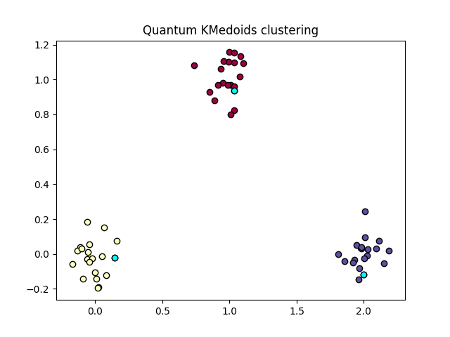
Example:

The following example shows how to use the QKMedoids class for clustering a synthetic dataset.

Note

The example requires the following additional dependencies:

• tno.quantum.ml.datasets: Used for the generation of artificial dataset.

• tno.quantum.optimization.qubo.solvers: Provides the specific QUBO solvers. In this example solvers from [dwave] are used.

Both can be installed alongside with the package by providing the [example] flag:: Both can be installed alongside with the package by providing the [example] flag:

pip install tno.quantum.ml.clustering.kmedoids[example]

Generate sample data:

>>> from tno.quantum.ml.datasets import get_blobs_clustering_dataset
>>> n_centers = 3
>>> X, true_labels = get_blobs_clustering_dataset(
...     n_samples=60, n_features=2, n_centers=n_centers
... )

Create QKMedoids object and fit:

>>> from tno.quantum.ml.clustering.kmedoids import QKMedoids
>>> cobj = QKMedoids(
...     n_clusters=n_centers,
...     solver_config={
...         "name": "simulated_annealing_solver",
...         "options": {"random_state": 42, "num_read": 1000, "num_sweeps": 2000},
...     },
... )
>>> pred_labels = cobj.fit_predict(X)

Plot results:

>>> import matplotlib.pyplot as plt
>>> import numpy as np
>>> fig, ax = plt.subplots()
>>> unique_labels = np.unique(pred_labels)
>>> colors = plt.cm.Spectral(np.linspace(0, 1, len(unique_labels)))
>>> for k, col in zip(unique_labels, colors):
...     mask = cobj.labels_ == k
...     x, y = X[mask].T
...     ax.plot(x, y, "o", mfc=col, mec="k", ms=6)
>>> x_centers, y_centers = cobj.cluster_centers_.T
>>> ax.plot(x_centers, y_centers, "o", mfc="cyan", mec="k", ms=6)
>>> ax.set_title("Quantum KMedoids clustering")
>>> plt.savefig("/tmp/qkmedoids.png")

class tno.quantum.ml.clustering.kmedoids.QKMedoids(n_clusters=2, alpha=1, beta=1, gamma=2, metric='euclidean', solver_config=None)

Bases: ClusterMixin, QUBOEstimator

Quantum K-medoid clustering.

__init__(n_clusters=2, alpha=1, beta=1, gamma=2, metric='euclidean', solver_config=None)

Init QKMedoid clustering algorithm.

The QKMedoid algorithm minimizes a double objective function with a constraint translated to a QUBO formulation. The first objective maximizes the distance between the medoids, while the second objective tries to make the medoid as centrally positioned as possible. The constraint restricts the number of medoids to be exactly equal to \(k\). The QUBO is an implementation of the work shown in [1] and [2]. Its cost function is given by:

\[\sum_{i=1}^N\sum_{j=1}^Nz_iz_j\left(\gamma-\frac{1}{2}\alpha\Delta_{ij}\right) + \sum_{i=1}^Nz_i\left(\beta\sum_{j=1}^N\Delta_{ij}-2\gamma k\right).\]

Details:

• \(z_{i}\) are the binary decision variables.

• \(N\) is the number of datapoints.

• \(k\) is the number of clusters.

• \(\Delta_{ij}=1-\exp(-\frac{1}{2}d_{ij})\), where \(d_{ij}\) is the distance between data point \(i\) and \(j\).

• \(\alpha\) is the weight parameter of the first objective, i.e., maximizing the distance between the medoids.

• \(\beta\) is the weight parameter of the second objective, i.e., centralizing the medoids.

• \(\gamma\) is the penalty parameter for the constraint that there must be exactly \(k\) medoids.

Parameters:

• n_clusters (SupportsInt) – The number of clusters to form (\(k\)). Must be a strictly positive integer value.

• alpha (SupportsFloat) – Weight parameter for identifying far apart points. The weight is scaled by 1 / (number of clusters). Must be non-negative and defaults to 1.

• beta (SupportsFloat) – Weight parameter for identifying central points. The weight is scaled by 1 / (number of samples). Must be non-negative and defaults to 1.

• gamma (SupportsFloat) – Penalty parameter for the constraint that the solution contains exactly the specified number of clusters (\(k\)).The penalty is scaled by \(\max_{i,j}\left(1-\exp(-\frac{1}{2}d_{ij})\right)\), where \(d_{ij}\) is the distance between data point \(i\) and \(j\). Must be non-negative and defaults to 2.

• metric (str | Callable[ArrayLike, ArrayLike, float]) – The metric to use when calculating distance between instances in a feature array, see sklearn.metrics.pairwise_distances(). If metric is a string, it must be one of the options allowed by scipy.spatial.distance.pdist(). If metric is "precomputed", X is assumed to be a distance matrix. If metric is a callable function, it is called on each pair of instances and the resulting values. The callable should take two arrays from X as input and return a value indicating their distance.

• solver_config (UnionType[SolverConfig, Mapping[str, Any], None]) – A QUBO solver configuration or None. In the former case includes name and options. If None is given, the default solver configuration as defined in get_default_solver_config_if_none() will be used. Default is None.

distance_

2-D array of shape (n_features, n_features) containing the pairwise distances between each feature vector.

medoid_indices_

1-D array of length n_clusters containing the indices of the medoid row in the feature matrix \(X\).

cluster_centers_

2-D array of shape (n_cluster, n_features) containing the cluster centers (elements from original dataset \(X\)).

labels_

1-D array of length n_samples containing the assigned labels for each sample.

inertia_

The sum of distances of samples to their closest cluster center.

__sklearn_tags__()

Return estimator tags.

Return type:

Tags

fit(X, y=None)

Fit the model to data matrix X.

Parameters:

• X (ArrayLike) – The input data.

• y (Optional[ArrayLike]) – Ignored.

Return type:

TypeVar(QKMedoidsT, bound= QKMedoids)

Returns:

Returns self, a trained QKMedoids class.