problems.portfolio_optimization
Multi-objective portfolio optimization using QUBO formulation.
This package provides Python code that converts a multi-objective portfolio optimization problem into a QUBO problem. The transformed problem can then be solved using quantum annealing techniques.
The following objectives can be considered
return on capital, indicated by ROC,
diversification, indicated by the Herfindahl-Hirschman Index HHI.
Additionally, we allow for capital growth factor and arbitrary emission reduction constraints to be considered.
Usage example:
>>> import numpy as np
>>> from tno.quantum.problems.portfolio_optimization import PortfolioOptimizer
>>> from tno.quantum.optimization.qubo import SolverConfig
>>>
>>> # Choose sampler for solving qubo
>>> solver_config = SolverConfig(
...     name="simulated_annealing_solver",
...     options={"num_reads": 20, "num_sweeps": 200, "random_state": 42},
... )
>>>
>>> # Set up penalty coefficients for the constraints
>>> lambdas1 = np.logspace(-16, 1, 25, endpoint=False, base=10.0)
>>> lambdas2 = np.logspace(-16, 1, 25, endpoint=False, base=10.0)
>>> lambdas3 = np.array([1])
>>>
>>> # Create portfolio optimization problem
>>> portfolio_optimizer = PortfolioOptimizer("benchmark_dataset")
>>> portfolio_optimizer.add_minimize_hhi(weights=lambdas1)
>>> portfolio_optimizer.add_maximize_roc(formulation=1, weights_roc=lambdas2)
>>> portfolio_optimizer.add_emission_constraint(
...     weights=lambdas3,
...     emission_now="emis_intens_now",
...     emission_future="emis_intens_future",
...     name="emission",
... )
>>>
>>> # Solve the portfolio optimization problem
>>> results = portfolio_optimizer.run(solver_config, verbose=True)
>>> print(results.head())
                                  outstanding amount  diff ROC  diff diversification  diff outstanding  diff emission
0  (14.0, 473.0, 26.666666666666668, 1410.0, 74.0...  4.105045             -6.102454          1.514694     -29.999998
1  (19.0, 473.0, 28.0, 1196.6666666666667, 68.0, ...  2.574088             -2.556330          1.520952     -29.999992
2  (17.333333333333332, 509.6666666666667, 24.0, ...  2.979830             -6.397679          1.566499     -29.999988
3  (15.666666666666666, 491.3333333333333, 25.333...  1.875721             -4.025964          1.531100     -30.000023
4  (15.666666666666666, 491.3333333333333, 24.0, ...  2.697235             -7.117611          1.555159     -29.999977
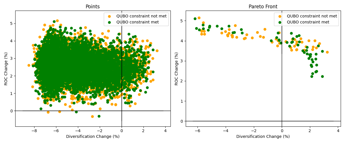
The Pareto front, the set of solutions where one objective can’t be improved without worsening the other objective, can be computed for return on capital and diversification.
>>> import matplotlib.pyplot as plt
>>> from tno.quantum.problems.portfolio_optimization import plot_front, plot_points
>>>
>>> (x1, y1), (x2, y2) = results.slice_results()
>>> fig, (ax1, ax2) = plt.subplots(ncols=2, figsize=(12, 5))
>>>
>>> # Plot data points
>>> plot_points(x2, y2, color="orange", label="QUBO constraint not met", ax=ax1)
>>> plot_points(x1, y1, color="green", label="QUBO constraint met", ax=ax1)
>>> ax1.set_title("Points")
>>>
>>> # Plot Pareto front
>>> plot_front(x2, y2, color="orange", label="QUBO constraint not met", ax=ax2)
>>> plot_front(x1, y1, color="green", label="QUBO constraint met", ax=ax2)
>>> ax2.set_title("Pareto Front")
>>> fig.tight_layout()
>>> plt.show()
Data input
The data used for the portfolio optimization can be imported via an excel file, csv file,
json file or as a Pandas DataFrame.
The data needs to contain at least the following columns:
asset: The name of the asset.
outstanding_now: Current outstanding amount per asset.
min_outstanding_future: Lower bound outstanding amount in the future per asset.
max_outstanding_future: Upper bound outstanding amount in the future per asset.
income_now: Current income per asset, corresponds to return multiplied by the current outstanding amount.
regcap_now: Current regulatory capital per asset.
The table below shows an example dataset with the correct structure. Note that this is the least amount of columns that need to be present. More columns are allowed and required for some functionalities.
asset |
outstanding_now |
min_outstanding_future |
max_outstanding_future |
income_now |
regcap_now |
|---|---|---|---|---|---|
Sector 1 COUNTRY 1 |
10 |
14 |
19 |
5 |
5 |
Sector 2 COUNTRY 1 |
600 |
473 |
528 |
70 |
40 |
Sector 3 COUNTRY 1 |
20 |
24 |
28 |
5 |
10 |
Sector 4 COUNTRY 1 |
800 |
1090 |
1410 |
1 |
2 |
Sector 1 COUNTRY 2 |
40 |
56 |
74 |
10 |
5 |
Sector 2 COUNTRY 2 |
200 |
291 |
397 |
40 |
20 |
… |
… |
… |
… |
… |
… |
If the input data file contains the correct information but has different column names,
you can rename the columns without modifying the input file. For more details and
examples, refer to the documentation of
PortfolioData.
The codebase is based on the following paper:
- class tno.quantum.problems.portfolio_optimization.PortfolioData(portfolio_dataframe, columns_rename=None)[source]
Bases:
objectThe
PortfolioDatastores the data used for portfolio optimization.The example below shows how to load and print info for a benchmark dataset.
>>> from tno.quantum.problems.portfolio_optimization import PortfolioData
>>> portfolio_data = PortfolioData.from_file("benchmark_dataset")
>>> portfolio_data.print_portfolio_info()
PortfolioData: --------- Portfolio information -----------
PortfolioData: Total outstanding now: 21252.70
PortfolioData: ROC now: 1.0642
PortfolioData: HHI now: 1.0000
PortfolioData: Total Emission now: 43355508.00
PortfolioData: Relative emission intensity now: 2040.00
PortfolioData: Expected total outstanding future: 31368.00
PortfolioData: Std dev: 886.39
PortfolioData: Expected average growth factor: 1.4760
PortfolioData: Std dev: 0.0417
PortfolioData: --------- --------------------- -----------
- __init__(portfolio_dataframe, columns_rename=None)[source]
Creates a
PortfolioDataobject from a pandasDataFrame.The portfolio data is expected to contain at least the following columns names:
"assets": The name of the asset."outstanding_now_now": Current outstanding amount per asset."min_outstanding_future": Lower bound outstanding amount in the future per asset."max_outstanding_future": Upper bound outstanding amount in the future per asset."income_now": Current income per asset, corresponds to return multiplied by the current outstanding amount."regcap_now": Current regulatory capital per asset.
Different column names in the dataset can be used, but in that case they need to be provided as a renaming dictionary to the
columns_renameargument.- Parameters:
- Raises:
ValueError if required columns are not present in dataset. –
- __str__()[source]
String representation of the
PortfolioDataobject.- Return type:
- classmethod from_file(filename, columns_rename=None)[source]
Reads portfolio data object into
PortfolioData.The portfolio data is expected to contain at least the following columns names:
"assets": The name of the asset."outstanding_now_now": Current outstanding amount per asset."min_outstanding_future": Lower bound outstanding amount in the future per asset."max_outstanding_future": Upper bound outstanding amount in the future per asset."income_now": Current income per asset, corresponds to return multiplied by the current outstanding amount."regcap_now": Current regulatory capital per asset.
Different column names in the dataset can be used, but in that case they need to be provided as a renaming dictionary to the
columns_renameargument.- Parameters:
filename (
str|Path) – path to portfolio data. If insteadbenchmark_datasetis provided, a default benchmark dataset containing 52 assets will be used.columns_rename (
dict[str,str] |None) – to rename columns provided as dict with new column names as keys and to replace column name as value. Example{"outstanding_2021": "outstanding_now"}.
- Raises:
ValueError if required columns are not present in dataset. –
- Return type:
TypeVar(PortfolioDataT, bound= PortfolioData)
- class tno.quantum.problems.portfolio_optimization.PortfolioOptimizer(portfolio_data, k=2, columns_rename=None)[source]
Bases:
objectClass to perform portfolio optimization.
The
PortfolioOptimizerclass is used to convert multi-objective portfolio optimization problems into QUBO problems which can then be solved using QUBO solving techniques such as simulated or quantum annealing.The following objectives can be considered
return on capital, indicated by ROC,
diversification, indicated by the Herfindahl-Hirschman Index HHI.
The following constraints can be added
capital growth, demand a minimum increase in outstanding assets.
emission reduction, demand a minimum reduction for an arbitrary emission type.
- __init__(portfolio_data, k=2, columns_rename=None)[source]
Init
PortfolioOptimizer.- Parameters:
portfolio_data (
PortfolioData|DataFrame|str|Path) – Portfolio data represented by either the portfolio data object, pandas dataframe or path to where portfolio data is stored. See the docstring ofPortfolioDatafor data input conventions.k (
int) – The number of bits that are used to represent the outstanding amount for each asset. A fixed point representation is used to represent \(2^k\) different equidistant values in the range \([LB_i, UB_i]\) for asset i.columns_rename (
dict[str,str] |None) – can be used to rename data columns. See the docstring ofPortfolioDatafor an example.
- Raises:
TypeError – If the provided portfolio data input has the wrong type.
- add_emission_constraint(emission_now, emission_future=None, reduction_percentage_target=0.7, name=None, weights=None)[source]
Adds emission constraint to the portfolio optimization problem.
The constraint is given by
\[\frac{\sum_{i=1}^Nf_i \cdot x_i}{\sum_{i=1}^N x_i} = g_e \frac{\sum_{i=1}^Ne_i \cdot y_i}{\sum_{i=1}^N y_i},\]where:
\(N\) is the total number of assets,
\(x_i\) is the future outstanding amount for asset \(i\),
\(y_i\) is the current outstanding amount for asset \(i\),
\(e_i\) is the current emission intensity for asset \(i\),
\(f_i\) is the expected emission intensity at the future for asset \(i\),
\(g_e\) is the target value for the relative emission reduction.
Usage example:
>>> from tno.quantum.problems.portfolio_optimization import PortfolioOptimizer
>>> import numpy as np
>>> portfolio_optimizer = PortfolioOptimizer(portfolio_data="benchmark_dataset")
>>> lambdas = np.logspace(-16, 1, 25, endpoint=False, base=10.0)
>>> portfolio_optimizer.add_emission_constraint(
...   emission_now="emis_intens_now", weights=lambdas
... )
For the QUBO formulation, see the docs of
calc_emission_constraint().- Parameters:
emission_now (
str) – Name of the column in the portfolio dataset corresponding to the variables emission intensity at current time.emission_future (
str|None) – Name of the column in the portfolio dataset corresponding to the variables emission intensity at future time. If no value is provided, it is assumed that the emission intensity is constant over time, i.e., the variableemission_nowwill be used.reduction_percentage_target (
float) – target value for reduction percentage amount.name (
str|None) – Name that will be used for emission constraint in the results df.weights (
Optional[ArrayLike]) – The coefficients that are considered as penalty parameter.
- Return type:
- add_growth_factor_constraint(growth_target, weights=None)[source]
Adds outstanding amount growth factor constraint to optimization problem.
The constraint is given by
\[\frac{\sum_{i=1}^N x_i}{\sum_{i=1}^N y_i} = g_c,\]where
\(N\) is the total number of assets,
\(x_i\) is the future outstanding amount for asset \(i\),
\(y_i\) is the current outstanding amount for asset \(i\),
\(g_c\) is the target value for the total growth factor.
This constraint can only be added once.
Usage example:
>>> from tno.quantum.problems.portfolio_optimization import PortfolioOptimizer
>>> import numpy as np
>>> portfolio_optimizer = PortfolioOptimizer(portfolio_data="benchmark_dataset")
>>> lambdas = np.logspace(-16, 1, 25, endpoint=False, base=10.0)
>>> portfolio_optimizer.add_growth_factor_constraint(growth_target=1.2, weights=lambdas)
For the QUBO formulation, see the docs of
calc_growth_factor_constraint().- Parameters:
growth_target (
float) – target value for growth factor total outstanding amount.weights (
Optional[ArrayLike]) – The coefficients that are considered as penalty parameter.
- Raises:
ValueError – If constraint has been added before.
- Return type:
- add_maximize_roc(formulation, weights_roc=None, ancilla_variables=0, weights_stabilize=None)[source]
Adds the maximize ROC objective to the portfolio optimization problem.
The ROC objective is given by
\[ROC(x) = \frac{\sum_{i=1}^N \frac{x_i \cdot r_i}{y_i}} {\sum_{i=1}^N \frac{x_i \cdot c_i}{y_i}},\]where
\(N\) is the total number of assets,
\(x_i\) is the future outstanding amount for asset \(i\),
\(y_i\) is the current outstanding amount for asset \(i\),
\(r_i\) is the return for asset \(i\),
\(c_i\) is the regulatory capital for asset \(i\).
As the ROC is not a quadratic function, it is approximated using two different formulations:
- formulation 1:
- \[ROC_1(x)=\sum_{i=1}^N\frac{x_i\cdot r_i}{c_i\cdot y_i}\]
Adds 1 qubo term, use
weights_rocto scale. - formulation 2:
- \[ROC_2(x)=\frac{1}{G_C \cdot C_{21}}\sum_{i=1}^N x_i\frac{r_i}{y_i}\]
In this formulation, \(G_C \cdot C_{21}\) approximates a fixed regulatory capital growth which is equal for all assets, where
\(1≤G_C<2\) is a growth factor to be estimated using ancilla variables,
\(C_{21} = \sum_{i=1}^N c_{i}\) is the sum of all assets’ regulatory capital.
This formulation adds 2 qubo terms, one for the ROC term, and one to stabilize the capital growth. The stabilize qubo requires an extra argument
ancilla_variables. Useweights_rocandweights_stabilizeto scale both qubo’s accordingly.
For the QUBO formulation, see the docs of
calc_maximize_roc1()andcalc_maximize_roc2().Usage example:
>>> from tno.quantum.problems.portfolio_optimization import PortfolioOptimizer
>>> import numpy as np
>>> portfolio_optimizer = PortfolioOptimizer(portfolio_data="benchmark_dataset")
>>> lambdas = np.logspace(-16, 1, 25, endpoint=False, base=10.0)
>>> portfolio_optimizer.add_maximize_roc(formulation=1, weights_roc=lambdas)
- Parameters:
formulation (
int) – the ROC QUBO formulation that is being used. Possible options are: [1, 2].weights_roc (
Optional[ArrayLike]) – The coefficients that are considered as penalty parameter for maximizing the roc objective.ancilla_variables (
int) – The number of ancillary variables that are used to representG_Cusing fixed point representation. Only relevant for roc formulation2.weights_stabilize (
Optional[ArrayLike]) – The coefficients that are considered as penalty parameter for the stabilizing constraint. Only relevant for roc formulation2.
- Raises:
ValueError – If invalid formulation is provided.
- Return type:
- add_minimize_hhi(weights=None)[source]
Adds the minimize HHI objective to the portfolio optimization problem.
The HHI objective is given by
\[HHI(x) = \sum_{i=1}^N\left(\frac{x_i}{\sum_{j=1}^N x_j}\right)^2,\]where
\(N\) is the total number of assets,
\(x_i\) is the future outstanding amount for asset \(i\).
As the objective contains non-quadratic terms, a QUBO formulation requires approximations. For the QUBO formulation, see the docs of
calc_minimize_hhi().Usage example:
>>> from tno.quantum.problems.portfolio_optimization import PortfolioOptimizer
>>> import numpy as np
>>> portfolio_optimizer = PortfolioOptimizer(portfolio_data="benchmark_dataset")
>>> lambdas = np.logspace(-16, 1, 25, endpoint=False, base=10.0)
>>> portfolio_optimizer.add_minimize_hhi(weights=lambdas)
- Parameters:
weights (
Optional[ArrayLike]) – The coefficients that are considered as penalty parameter.- Return type:
- run(solver_config=None, *, verbose=True)[source]
Optimizes a portfolio given the set of provided constraints.
Usage example:
>>> from tno.quantum.problems.portfolio_optimization import PortfolioOptimizer
>>> portfolio_optimizer = PortfolioOptimizer(portfolio_data="benchmark_dataset")
>>> portfolio_optimizer.add_minimize_hhi()
>>> portfolio_optimizer.run()
- Parameters:
solver_config (
SolverConfig|Mapping[str,Any] |None) – Configuration for the qubo solver to use. Must be aSolverConfigor a mapping with"name"and"options"keys. IfNone(default) is provided, the``{"name": "simulated_annealing_solver", "options": {}}`.verbose (
bool) – If True, print detailed information during execution
- Return type:
Results- Returns:
Results.
- Raises:
ValueError – if constraints are not set
- class tno.quantum.problems.portfolio_optimization.QuboFactory(portfolio_data, k)[source]
Bases:
objectQuboFactory - A factory class for creating
QUBOinstances.This class provides a convenient interface for constructing intermediate QUBO matrices for different objectives and constraints.
calc_minimize_hhi: Calculates the to minimize HHI QUBO.
calc_maximize_roc1: Calculates the to maximize return on capital QUBO variant 1.
calc_maximize_roc2: Calculates the to maximize return on capital QUBO variant 2.
calc_emission_constraint: Calculates the emission constraint QUBO.
calc_growth_factor_constraint: Calculates the growth factor constraint QUBO.
calc_stabilize_c: Calculates the constraint QUBO that stabilizes growth factor.
- __init__(portfolio_data, k)[source]
Init of the
QuboFactory.- Parameters:
portfolio_data (
PortfolioData) – Data of the portfolio to optimize.k (
int) – The number of bits that are used to represent the outstanding amount for each asset. A fixed point representation is used to represent \(2^k\) different equidistant values in the range \([LB_i, UB_i]\) for asset i.
- calc_emission_constraint(emission_now, emission_future=None, reduction_percentage_target=0.7)[source]
Calculate emission constraint QUBO for arbitrary reduction target.
The QUBO formulation is given by
\[ \begin{align}\begin{aligned}QUBO(x) &= \left( \sum_{i=1}^N f_i x_i - g_e E \sum_{i=1}^N x_i \right)^2,\\x_i & = LB_i+\frac{UB_i-LB_i}{2^k-1}\sum_{j=0}^{k-1}2^j\cdot x_{i,j},\\E &= \frac{\sum_{i=1}^N e_i \cdot y_i}{\sum_{i=1}^N y_i},\end{aligned}\end{align} \]where:
\(LB_i\) is the lower bound for asset \(i\),
\(UB_i\) is the upper bound for asset \(i\),
\(k\) is the number of bits,
\(e_i\) is the current emission intensity for asset \(i\),
\(f_i\) is the expected emission intensity at the future for asset \(i\),
\(y_i\) is the current outstanding amount for asset \(i\),
\(g_e\) is the target value for the relative emission reduction,
and \(x_{i,j}\) are the \(k\) binary variables for asset \(i\) with \(j<k\).
- Parameters:
emission_now (
str) – Name of the column in the portfolio dataset corresponding to the variables at current time.emission_future (
str|None) – Name of the column in the portfolio dataset corresponding to the variables at future time. If no value is provided, it is assumed that the value is constant over time, i.e., the variableemission_nowwill be used.reduction_percentage_target (
float) – Target value for reduction percentage amount.
- Raises:
KeyError – if the provided column names are not in the portfolio_data.
- Return type:
- Returns:
The QUBO.
- calc_growth_factor_constraint(growth_target)[source]
Calculates the growth factor constraint QUBO.
The QUBO formulation is given by
\[QUBO(x) = \left( \frac{\sum_{i=1}^N LB_i + \frac{UB_i-LB_i}{2^k-1}\sum_{j=0}^{k-1} 2^j\cdot x_{i,j}}{\sum_{i=1}^N y_i} - g_c \right)^2\]where:
\(LB_i\) is the lower bound for asset \(i\),
\(UB_i\) is the upper bound for asset \(i\),
\(k\) is the number of bits,
\(g_c\) is the target value for the total growth factor,
\(y_i\) is the current outstanding amount for asset \(i\),
and \(x_{i,j}\) are the \(k\) binary variables for asset \(i\) with \(j<k\).
- calc_maximize_roc1()[source]
Calculates the to maximize ROC QUBO for variant 1.
The QUBO formulation is given by
\[QUBO(x) = -\sum_{i=1}^N\frac{r_i}{c_i\cdot y_i} \left(LB_i + \frac{UB_i-LB_i}{2^k-1}\sum_{j=0}^{k-1}2^j\cdot x_{i,j}\right),\]where
\(LB_i\) is the lower bound for asset \(i\),
\(UB_i\) is the upper bound for asset \(i\),
\(k\) is the number of bits,
\(y_i\) is the current outstanding amount for asset \(i\),
\(r_i\) is the current return for asset \(i\),
\(c_i\) is the regulatory capital for asset \(i\),
and \(x_{i,j}\) are the \(k\) binary variables for asset \(i\) with \(j<k\).
- Return type:
- Returns:
The QUBO.
- calc_maximize_roc2()[source]
Calculates the to maximize ROC QUBO for variant 2.
The QUBO formulation is given by
\[ \begin{align}\begin{aligned}QUBO(x,g) &= - G_{inv}(g) \cdot \sum_{i=1}^N\frac{r_i}{y_i} \left(LB_i + \frac{UB_i-LB_i}{2^k-1}\sum_{j=0}^{k-1}2^j\cdot x_{i,j}\right),\\G_{inv}(g) &= 1 + \sum_{j=0}^{k-1} 2^{-j-1}(2^{-j-1} - 1)\cdot g_{j},\end{aligned}\end{align} \]where
\(LB_i\) is the lower bound for asset \(i\),
\(UB_i\) is the upper bound for asset \(i\),
\(k\) is the number of bits,
\(a\) is the number of ancilla variables,
\(y_i\) is the current outstanding amount for asset \(i\),
\(r_i\) is the return for asset \(i\),
\(c_i\) is the regulatory capital for asset \(i\),
\(x_{i,j}\) are the \(k\) binary variables for asset \(i\) with \(j<k\).
\(g_{j}\) are the \(a\) binary ancilla variables with \(j<a\).
- Return type:
- Returns:
The QUBO.
- calc_minimize_hhi()[source]
Calculates the to minimize HHI QUBO.
The QUBO formulation is given by
\[QUBO(x) = \sum_{i=1}^N\left(LB_i + \frac{UB_i-LB_i}{2^k-1}\sum_{j=0}^{k-1}2^j\cdot x_{i,j}\right)^2,\]where:
\(LB_i\) is the lower bound for asset \(i\),
\(UB_i\) is the upper bound for asset \(i\),
\(k\) is the number of bits,
and \(x_{i,j}\) are the \(k\) binary variables for asset \(i\) with \(j<k\).
- Return type:
- Returns:
The QUBO.
- calc_stabilize_c()[source]
Calculate QUBO that stabilizes the growth factor in second ROC formulation.
The QUBO formulation is given by
\[ \begin{align}\begin{aligned}QUBO(x,g) &= \left( \sum_{i=1}^N\frac{c_i}{y_i} \left(LB_i + \frac{UB_i-LB_i}{2^k-1}\sum_{j=0}^{k-1}2^j\cdot x_{i,j}\right) - G_C(g)\sum_{i=1}^N c_i \right)^2,\\G_C &= 1 + \sum_{j=0}^{k-1} 2^{-j - 1} \cdot g_j,\end{aligned}\end{align} \]where
\(LB_i\) is the lower bound for asset \(i\),
\(UB_i\) is the upper bound for asset \(i\),
\(k\) is the number of bits,
\(a\) is the number of ancilla variables,
\(y_i\) is the current outstanding amount for asset \(i\),
\(c_i\) is the regulatory capital for asset \(i\),
\(x_{i,j}\) are the \(k\) binary variables for asset \(i\) with \(j<k\),
\(g_j\) are the \(a\) ancillary binary variables with \(j<a\).
- Return type:
- Returns:
The QUBO.
- tno.quantum.problems.portfolio_optimization.plot_front(diversification_values, roc_values, color=None, label=None, c=None, vmin=None, vmax=None, alpha=None, cmap=None, ax=None)[source]
Plots a pareto front of the given data-points in a Diversification-ROC plot.
- Parameters:
diversification_values (
ArrayLike) – 1-DArrayLikecontaining the x values of the plot.roc_values (
ArrayLike) – 1-DArrayLikecontaining the y values of the plot.color (
str|None) – Optional color to use for the points. For an overview of allowed colors see the Matplotlib Documentation. IfNoneis given, a default color will be assigned bymatplotlib. Default isNone.label (
str|None) – Label to use in the legend. IfNoneis given, no label will be used. Default isNone.c (
Union[_Buffer,_SupportsArray[dtype[Any]],_NestedSequence[_SupportsArray[dtype[Any]]],complex,bytes,str,_NestedSequence[complex|bytes|str],Sequence[tuple[float,float,float] |str|tuple[float,float,float,float] |tuple[tuple[float,float,float] |str,float] |tuple[tuple[float,float,float,float],float]],tuple[float,float,float],tuple[float,float,float,float],tuple[tuple[float,float,float] |str,float],tuple[tuple[float,float,float,float],float],None]) – The marker colors as used bymatplotlib.vmin (
float|None) – min value of data range that colormap covers as used bymatplotlib.vmax (
float|None) – max value of data range that colormap covers as used bymatplotlib.alpha (
float|None) – The alpha blending value as used bymatplotlib.cmap (
str|Colormap|None) – Colormap instance or registered colormap name as used bymatplotlib.ax (
Axes|None) –Axesto plot on. IfNone, a new figure with oneAxeswill be created.
- Return type:
- Returns:
The
matplotlibPathCollection object created by scatter.
- tno.quantum.problems.portfolio_optimization.plot_points(diversification_values, roc_values, color=None, label=None, c=None, vmin=None, vmax=None, alpha=None, cmap=None, ax=None)[source]
Plots the given data-points in a Diversification-ROC plot.
- Parameters:
diversification_values (
ArrayLike) – 1-DArrayLikecontaining the x values of the plot.roc_values (
ArrayLike) – 1-DArrayLikecontaining the y values of the plot.color (
str|None) – Optional color to use for the points. For an overview of allowed colors see the Matplotlib Documentation. IfNoneis given, a default color will be assigned bymatplotlib. Default isNone.label (
str|None) – Label to use in the legend. IfNoneis given, no label will be used. Default isNone.c (
Union[_Buffer,_SupportsArray[dtype[Any]],_NestedSequence[_SupportsArray[dtype[Any]]],complex,bytes,str,_NestedSequence[complex|bytes|str],Sequence[tuple[float,float,float] |str|tuple[float,float,float,float] |tuple[tuple[float,float,float] |str,float] |tuple[tuple[float,float,float,float],float]],tuple[float,float,float],tuple[float,float,float,float],tuple[tuple[float,float,float] |str,float],tuple[tuple[float,float,float,float],float],None]) – The marker colors as used bymatplotlib.vmin (
float|None) – min value of data range that colormap covers as used bymatplotlib.vmax (
float|None) – max value of data range that colormap covers as used bymatplotlib.alpha (
float|None) – The alpha blending value as used bymatplotlib.cmap (
str|Colormap|None) – Colormap instance or registered colormap name as used bymatplotlib.ax (
Axes|None) –Axesto plot on. IfNone, a new figure with oneAxeswill be created.
- Return type:
- Returns:
The
matplotlibPathCollection object created by scatter.