Linear regression

This page contains advanced examples for the tno.quantum.ml.regression.linear_regression package. Examples of basic usage can be found in the module’s documentation.

Requirements

Install the following dependencies to run the examples below:

pip install tno.quantum.ml.regression.linear_regression
pip install seaborn

Examples

Example 1: Assume a linear system of the form \(Ax=b\) where:

• \(A\) is the training data.

• \(x\) is a vector of unknown coefficients.

• \(b\) is a vector of target values.

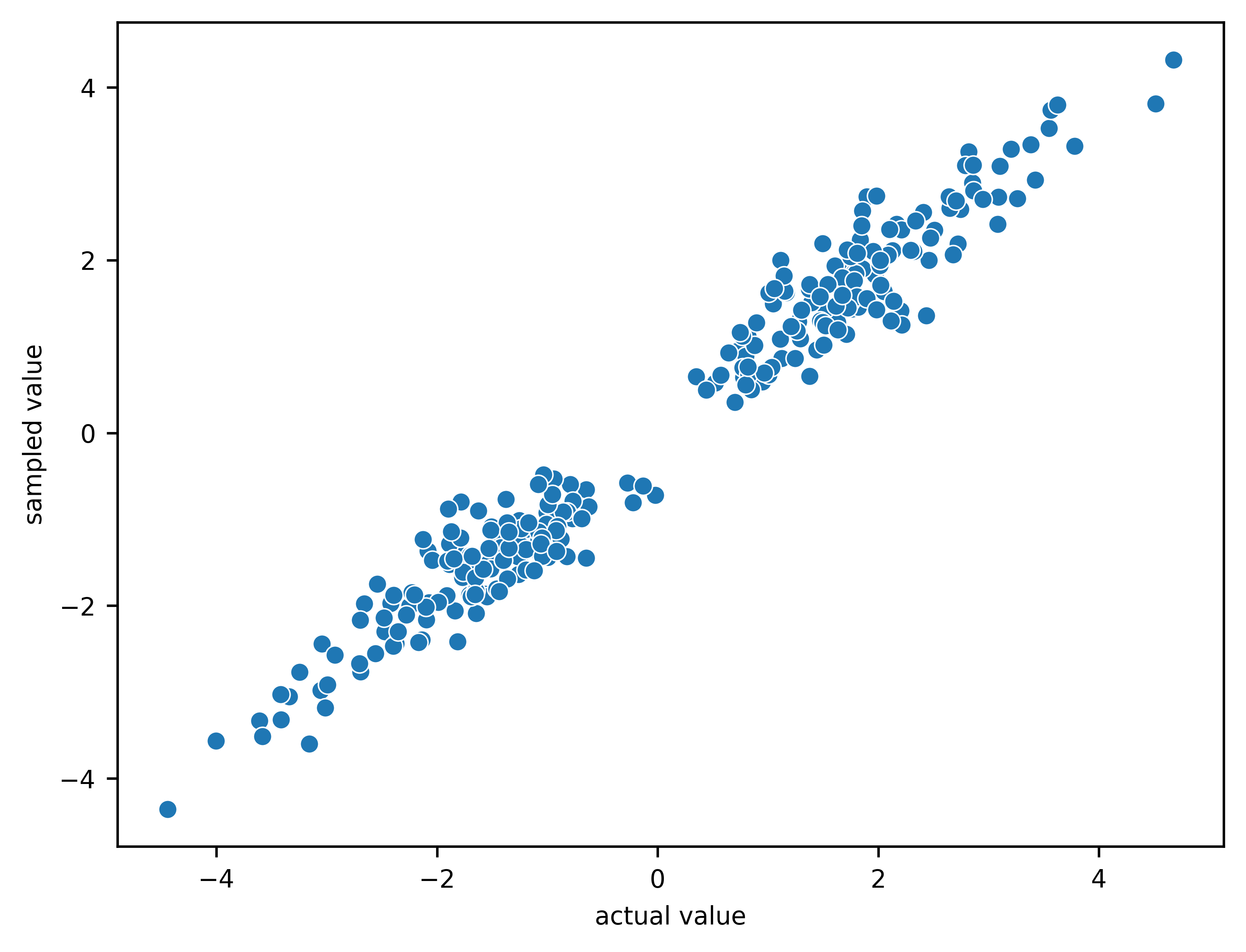
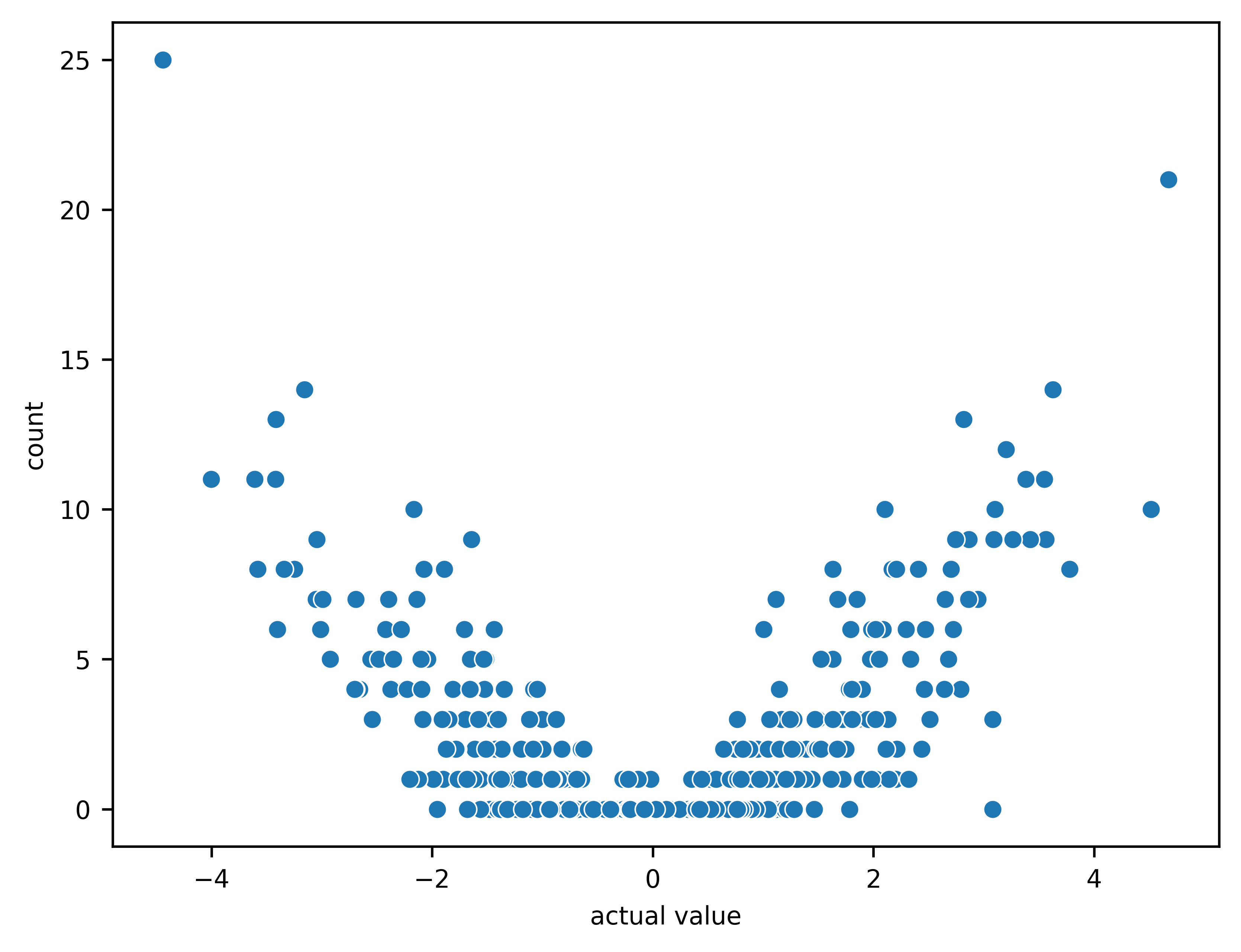
The following fits the model based on \(A\) and \(b\), and shows the following relationships:

• The sampled values (predictions) for \(b\) versus their actual values.

• The sampled values (predictions) for \(b\) versus their sampling count (i.e., the number of times the corresponding index has been sampled).

Note that larger values are sampled more often as expected.

import logging

import matplotlib as mpl
import numpy as np
import pandas as pd
import seaborn as sns

from tno.quantum.ml.regression.linear_regression import QILinearEstimator

mpl.use("Agg")
import matplotlib.pyplot as plt

plt.rcParams["font.size"] = "8"

logging.basicConfig(
    format="%(levelname)s:%(message)s", level=logging.INFO, datefmt="%Y-%m-%d %H:%M:%S"
)


def _save_fig(name: str) -> None:
    plt.savefig(name, dpi=600, bbox_inches="tight")
    plt.close("all")


def run_example() -> None:
    """Example of quantum-inspired linear prediction."""
    random_state = 111

    # Load data
    rank = 3
    m = 500
    n = 250
    rng = np.random.RandomState(random_state)
    A = rng.normal(0, 1, (m, n))
    U, S, V = np.linalg.svd(A, full_matrices=False)
    S[rank:] = 0
    A = U @ np.diag(S) @ V
    x = rng.normal(0, 1, A.shape[1])
    b = A @ x

    # Solve using quantum-inspired algorithm
    rank = 3
    r = 100
    c = 100
    n_samples = 100
    n_entries_b = 1000
    sketcher_name = "fkv"
    qi = QILinearEstimator(
        r, c, rank, n_samples, random_state, sketcher_name=sketcher_name
    )
    qi = qi.fit(A, b)
    sampled_indices, sampled_b = qi.sample_prediction_b(A, n_entries_b)

    # Process results
    df = pd.DataFrame({"b_idx_samples": sampled_indices, "b_samples": sampled_b})  # noqa: PD901
    df_counts = df.groupby("b_idx_samples")["b_idx_samples"].count()
    unique_sampled_indices = np.asarray(df_counts.keys())
    counts = np.asarray(df_counts.values)
    df_mean = df.groupby("b_idx_samples")["b_samples"].mean()
    unique_sampled_indices2 = np.asarray(df_mean.keys())
    unique_sampled_b = np.asarray(df_mean.values)
    assert np.all(unique_sampled_indices == unique_sampled_indices2)

    # Plot results
    b_counts = np.zeros(b.size)
    b_counts[unique_sampled_indices] = counts
    b_vs_sampled_counts_df = pd.DataFrame({"actual value": b, "count": b_counts})
    sns.scatterplot(data=b_vs_sampled_counts_df, x="actual value", y="count")
    _save_fig("example1-actual_value_vs_count")

    b_vs_avg_sampled_b_df = pd.DataFrame(
        {"actual value": b[unique_sampled_indices], "sampled value": unique_sampled_b}
    )
    sns.scatterplot(data=b_vs_avg_sampled_b_df, x="actual value", y="sampled value")
    _save_fig("example1-actual_value_vs_sampled_value")


if __name__ == "__main__":
    run_example()